Learning through Auxiliary Tasks

Play, a seemingly futile activity, is ubiquitous in human cultures and very widespread in the animal kingdom, which suggests it serves an important purpose

Update: this blog post was expanded into a paper with more explanations and additional experiments.

In this post, I’d like to illustrate how auxiliary tasks can be beneficial for machine learning. I’ll first define this notion, provide examples and show how these tasks are usually incorporated in the mathematical formulation of deep learning problems. I’ll then propose an alternative approach and present first experimental results for this approach.

Auxiliary Tasks in Machine Learning
Standard Approach for Deep Auxiliary Learning
An Alternative Approach
Comparison to Uweighted and Weighted Cosine
Experiments
Conclusion
References

Auxiliary Tasks in Machine Learning

In machine learning, auxiliary tasks are tasks we try to accomplish with the sole objective of better performing one or several primary tasks. This situation, referred to here as auxiliary learning, contrasts with multitask learning¹, for which we are genuinely interested in accomplishing well all tasks, and single task learning, for which only one task is considered.

	Tasks performed during training	Tasks considered when assessing performance
Single task learning	One task
Multitask learning	Several tasks
Auxiliary learning	One or several primary tasks, one or several auxiliary tasks	Primary tasks

Table 1. Auxiliary learning compared to single task learning and multitask learning

Let’s look at a striking example (Caruana et al., 1996) based on the Medis Pneumonia Database. This database contains 14,199 cases of patients diagnosed with pneumonia and hospitalized. It includes:

30 basic measurements (e.g. pulse);
35 lab results (e.g. blood counts);
the indication whether each patient survived or died.

Rich Caruana and his colleagues’ primary task was to identify patients that were more likely to survive and should then not be hospitalized. In this context, the lab results, available only after hospitalization, couldn’t be used as inputs. However, it was still possible to take advantage of them. Rich Caruana and his colleagues tried, as an auxiliary task, to predict the lab results based on the basic measurements. They thus reduced the error rate for their primary task by 5-10%.

Auxiliary learning has often been successfully applied in other settings, such as in the examples below:

Domain	Primary task	Auxiliary tasks	Source
Deep learning	Training a deep neural network	Reconstructing corrupted versions of the neural network’s inputs and the activations of its hidden layers to learn useful features	(Vincent et al., 2008)
Computer vision	Identifying facial landmarks on face pictures	Estimating head pose and predicting facial attributes (“wearing glasses”, “smiling” and “gender”)	(Zhang et al., 2014)
Computer vision	Detecting objects in indoor scenes	Predicting scene labels and evaluating depth and surface orientation at pixel level	(Mordan et al., 2018)
Sequence modelling	Training a recurrent neural network on very long sequences	Reconstructing or predicting short segments of the sequences	(Trinh et al., 2018)
Natural language processing	Performing a natural language processing task	Predicting words based on their neighborhood to learn efficient word representations	(Mikolov et al., 2013)
Reinforcement learning	Playing a video game	Modifying the image perceived by the agent and predicting short-term rewards	(Jaderberg et al., 2016)
Reinforcement learning	Playing a video game	Predicting the future state based on the current state and the current action	(Burda et al., 2018)

Table 2. Auxiliary learning has been successfully used in a variety of settings

Standard Approach for Deep Auxiliary Learning

For the sake of clarity, let’s consider only the case of a single primary task and a single auxiliary task (generalizing to an arbitrary number of primary and auxiliary tasks is straightforward). Let’s suppose further that these tasks correspond to the minimization of a primary loss $\mathcal{L}_{\text{primary}}$ and an auxiliary loss $\mathcal{L}_{\text{auxiliary}}$ .

In the context of deep learning, the standard approach² is to use a single neural network for both tasks, with shared layers followed by task-specific layers, and to apply a gradient descent-based method to minimize the weighted sum of the two losses $\mathcal{L} = \mathcal{L}_{\text{primary}} + \lambda \mathcal{L}_{\text{auxiliary}}$ .

The corresponding gradient is $\nabla\mathcal{L} = \nabla\mathcal{L}_{\text{primary}} + \lambda \nabla\mathcal{L}_{\text{auxiliary}}$ .

The underlying intuition is that minimizing $\mathcal{L}$ will lead to more meaningful representations in the shared layers and that these representations will be leveraged by the layers specific to the primary task.

In the standard multitask approach, $\lambda$ is a constant value³. Its purpose is to balance the primary task and the auxiliary task. $\lambda = 0$ corresponds to single task learning whereas increasing $\lambda$ gives more and more influence to the auxiliary task.

An Alternative Approach

The approach described above has provided very good empirical results. However, an auxiliary task may be unhelpful or even harmful for the primary task. The latter case, which is called negative transfer, is a central challenge of auxiliary learning.

Negative transfer

Figure 1. Left: a pathological example of negative transfer with an auxiliary task chosen so that $\mathcal{L}_{\text{auxiliary}} = -\mathcal{L}_{\text{primary}}$. In this case, $\nabla\mathcal{L} = 0$ (assuming $\lambda = 1$) and the network's parameters are never updated during gradient descent. Right: a less extreme situation in which $\nabla\mathcal{L}_{\text{auxiliary}}$ still cancels a significant part of $\nabla\mathcal{L}_{\text{primary}}$

Moreover, using a weighted average of $\mathcal{L}_{\text{primary}}$ and $\mathcal{L}_{\text{auxiliary}}$ suggests we’d be willing to tolerate a higher value of $\mathcal{L}_{\text{primary}}$ if it helped sufficiently decrease $\mathcal{L}_{\text{auxiliary}}$ . On the contrary, reducing the auxiliary loss is only looked for to the extent this contributes to reducing the primary loss.

To mitigate negative transfer and better reflect the fundamental asymmetry between the primary loss and the auxiliary loss, I suggest substituting $\nabla\mathcal{L}$ with:

$G = \nabla\mathcal{L}_{\text{primary}} + \lambda G_{\text{auxiliary}}$

where $G_{\text{auxiliary}}$ is:

as close as possible to $\nabla\mathcal{L}_{\text{auxiliary}}$ , to preserve the insights brought by the auxiliary task;
closer to $\nabla\mathcal{L}_{\text{primary}}$ than $-\nabla\mathcal{L}_{\text{primary}}$ , to avoid following a direction detrimental to the primary task.

Otherwise said, $G_{\text{auxiliary}}$ is the projection of $\nabla\mathcal{L}_{\text{auxiliary}}$ on the half-space of vectors whose cosine similarity with $\nabla\mathcal{L}_{\text{primary}}$ is positive. If a critical point of $\mathcal{L}_{\text{primary}}$ hasn’t been reached yet (i.e. if $\nabla\mathcal{L}_{\text{primary}} \neq \mathbf{0}$ ), this ensures that $\mathcal{L}_{\text{primary}}$ will decrease if the learning rate if small enough.

Projection of the auxiliary loss gradient

Figure 2. If $\nabla\mathcal{L}_{\text{primary}}$ and $\nabla\mathcal{L}_{\text{auxiliary}}$ form an obtuse angle, the component of $\nabla\mathcal{L}_{\text{auxiliary}}$ parallel to $\nabla\mathcal{L}_{\text{primary}}$ is cancelled to avoid increasing $\mathcal{L}_{\text{primary}}$. If not, $\nabla\mathcal{L}_{\text{auxiliary}}$ is kept as it is

Comparison to Uweighted and Weighted Cosine

This approach, referred below as projection, is analogous to two methods, unweighted cosine and weighted cosine, recently proposed for the same purpose (Du et al., 2018). Yunshu Du, Wojciech Czarnecki and their colleagues also suggest to adjust $\nabla\mathcal{L}_{\text{auxiliary}}$ :

Method	Adjusted auxiliary loss gradient $G_{\text{auxiliary}}$
Unweighted cosine	$\left\{\begin{array}{lll}\nabla\mathcal{L}_{\text{auxiliary}}&\mbox{if }\cos(\nabla\mathcal{L}_{\text{primary}},\nabla\mathcal{L}_{\text{auxiliary}}) \geq 0 \\ 0&\mbox{if }\cos(\nabla\mathcal{L}_{\text{primary}},\nabla\mathcal{L}_{\text{auxiliary}}) < 0\end{array}\right.$
Weighted cosine	$\max(0, \cos(\nabla\mathcal{L}_{\text{primary}},\nabla\mathcal{L}_{\text{auxiliary}})).\nabla\mathcal{L}_{\text{auxiliary}}$
Projection	$\nabla\mathcal{L}_{\text{auxiliary}} - \min(0, \nabla\mathcal{L}_{\text{auxiliary}}.\frac{\nabla\mathcal{L}_{\text{primary}}}{\|\|\nabla\mathcal{L}_{\text{primary}}\|\|}).\frac{\nabla\mathcal{L}_{\text{primary}}}{\|\|\nabla\mathcal{L}_{\text{primary}}\|\|}$

Table 3. Unweighted cosine and weighted cosine compared to the method proposed here

If $\nabla\mathcal{L}_{\text{primary}}$ and $\nabla\mathcal{L}_{\text{auxiliary}}$ form an acute angle, both projection and unweighted cosine leave $\nabla\mathcal{L}_{\text{auxiliary}}$ unchanged whereas weighted cosine reduces its norm with the cosine similarity of these vectors. In particular, weighted cosine strongly shrinks $\nabla\mathcal{L}_{\text{auxiliary}}$ when it becomes almost orthogonal to $\nabla\mathcal{L}_{\text{primary}}$ .

If $\nabla\mathcal{L}_{\text{primary}}$ and $\nabla\mathcal{L}_{\text{auxiliary}}$ form an obtuse angle, both unweighted cosine and weighted cosine just ignore $\nabla\mathcal{L}_{\text{auxiliary}}$ . In contrast, projection only negates the component of $\nabla\mathcal{L}_{\text{auxiliary}}$ which is collinear to $\nabla\mathcal{L}_{\text{primary}}$ .

Unweighted and weighted cosine

Figure 3. $\nabla\mathcal{L}_{\text{auxiliary}}$ transformed into $G_{\text{auxiliary}}$ by unweighted cosine (red) and weighted cosine (purple)

Even if projection and unweighted/weighted cosine are similar, their motivations are different:

(Du et al., 2018) explicitly tries to favor auxiliary tasks similar to the primary task. For example, weighted cosine completely ignores the auxiliary task when $\nabla\mathcal{L}_{\text{auxiliary}}$ and $\nabla\mathcal{L}_{\text{primary}}$ are orthogonal.
In my intuition, an auxiliary task’s purpose is to bring a new perspective. It should nudge us towards interesting regions of the parameter space we wouldn’t have explored with only the primary task in focus. Therefore we can try to negate the component of $\nabla\mathcal{L}_{\text{auxiliary}}$ which seems clearly harmful to our objective but we shouldn’t necessarily discard auxiliary tasks dissimilar to the primary task⁴.

Experiments

Let’s now look at some experiments. They were performed with Tensorflow and you can find the corresponding notebooks and additional results on GitHub.

Toy Experiments

We start with a minimalistic example to illustrate how substituting $\nabla\mathcal{L}_{\text{auxiliary}}$ with $G_{\text{auxiliary}}$ gives priority to the primary task while still allowing progress on the auxiliary task.

In the euclidean plane $\mathbb{R^2}$ , we try to find a point $(x, y)$ that, above all, minimizes the square distance to the unit circle and, only if it doesn’t increase this distance, also minimizes the square distance to point (2, 0).

Otherwise said, $\mathcal{L}_{\text{primary}} = (\sqrt{x^2+y^2}-1)^2$ and $\mathcal{L}_{\text{auxiliary}} = (x-2)^2+y^2$ .

This is a slight departure from the principle of auxiliary learning described above. Here we want to accomplish both the primary task and the auxiliary task even if the primary task is the absolute priority (performing the primary task alone would be too easy).

The solution of this problem is of course $(1, 0)$ and we try to reach it by using a gradient descent-based algorithm starting from point $(0, 2)$ with $\lambda = 0.1$ .

Adam trajectories

Figure 4. Trajectories with Adam

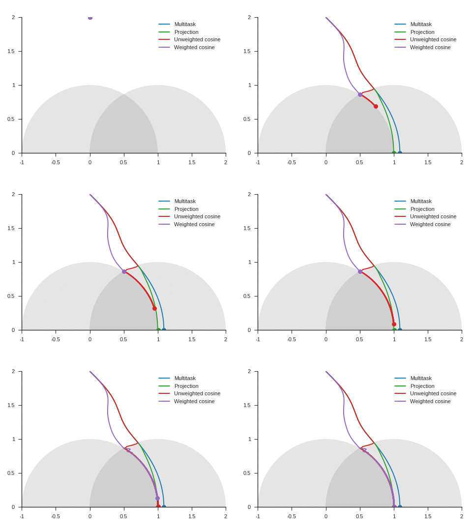
We can see the corresponding trajectories with the Adam algorithm (learning rate: 0.01, $\beta_1=0.9, \beta_2=0.999$ ) on Figure 4 and observe that:

With multitask, the point converges to a location close to but different from (1, 0) because of the distraction the auxiliary task creates.
With projection, the point follows as expected the same trajectory as with multitask before reaching the disk of radius 1 and center (1, 0), i.e. as long as $\nabla\mathcal{L}_{\text{primary}}$ and $\nabla\mathcal{L}_{\text{auxiliary}}$ form an acute angle. Afterwards, the point slightly deviates from the multitask trajectory to reach (1, 0).
The trajectory for unweighted cosine is also the same before reaching the disk of radius 1 and center (1, 0). Afterwards, the point abruptly changes course in the direction of the unit disk as the auxiliary task is ignored. When the point arrives at the unit disk, it starts oscillating around its edge. It’s then intermittently influenced by the auxiliary task and follows the unit circle until reaching (1, 0).
With weighted cosine, the point follows a more direct trajectory towards the unit circle. It then arrives close to the intersection between the unit circle and the circle of radius 1 and center (1, 0), i.e. a location where $\nabla\mathcal{L}_{\text{primary}}$ and $\nabla\mathcal{L}_{\text{auxiliary}}$ are orthogonal. It stagnates there for a while because the auxiliary task is mostly ignored then converges to (1, 0) by following the unit circle.

With this example, projection, unweighted cosine and weighted cosine allow to find the correct solution but the convergence is notably quicker with projection (this is also the case for other starting points).

Vanilla Gradient Descent trajectories

Figure 5. Trajectories with vanilla gradient descent

Figure 5 shows the trajectories with the vanilla gradient descent algorithm (learning rate: 0.01) and tells a different story. With unweighted cosine and weighted cosine, the point now stops on the unit circle far from (1, 0). This is because, in the absence of momentum, it eventually stays on the side of the unit circle where $\nabla\mathcal{L}_{\text{primary}}$ and $\nabla\mathcal{L}_{\text{auxiliary}}$ form an obtuse angle. The auxiliary task is then never taken into consideration anymore. A similar behavior can be seen with other starting points.

In summary, the proposed method works as intended with these toy examples: it helps accomplish both the primary task and the auxiliary task while giving precedence to the former.

Experiments on a Real Dataset

The following experiments are based on the CelebA (or large-scale CelebFaces attributes) dataset (Liu et al., 2015) and inspired by (Zhang et al., 2014). The CelebA dataset contains many face images annotated with 40 binary attributes such as Attractive, Young, Eyeglasses or Black Hair, and the locations of 5 facial landmarks : left eye, right eye, left mouth corner, right mouth corner and nose.

Example of a CelebA image

Figure 6. Examples of CelebA images and their 40 x 40 downsampled gray-scale versions with green dots on the 5 facial landmarks

The primary task for these experiments is to determine whether a face is attractive (or at least attractive in the annotators’ eyes) and the auxiliary task is to locate the facial landmarks. The corresponding losses are the cross entropy error function and the average quadratic error.

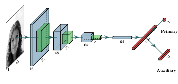
Neural network for the real dataset

Figure 7. Convolutional network with 4 convolutional layers interleaved with 3 max-pooling layers, a shared dense layer, and a final dense layer specific to each task

The pictures were downsampled to $40\times40$ and converted to gray-scale to make the tasks more challenging and reduce computation time. 10000 of them were included in the training set, the validation set and the test set. I used the neural network depicted on Figure 7 as in (Zhang et al., 2014) and trained it with the Adam algorithm and early stopping.

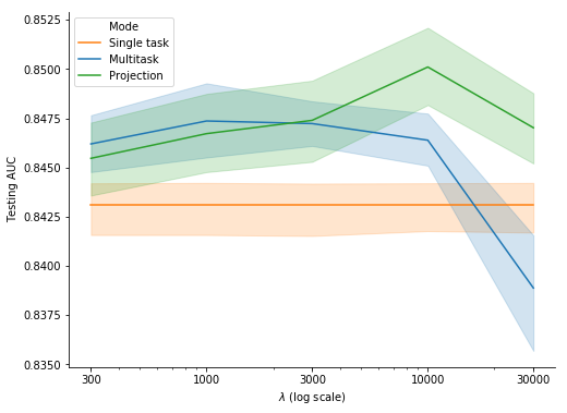
AUC for single task, multitask and projection

Figure 8. Testing AUC for single task, multitask and projection and 5 values of $\lambda$ (10 runs for each combination). The bands around the lines on this chart and the next ones correspond to the 95% confidence interval

Figure 8 shows the testing AUC for the primary task with single task, multitask and projection and various values of $\lambda$ :

Unsurprisingly enough, the multitask and projection curves get close to the single task curve as the influence of the auxiliary task becomes marginal for low values of $\lambda$ ;
The classification performance is better for multitask and projection than for single task for intermediate values of $\lambda$ . Moreover, the median testing AUC at the best $\lambda$ value for projection is slightly but statistically significantly higher than the one for multitask ( $p = 0.005$ with the Wilcoxon signed-rank test);
The classification performance deteriorates as the influence of the auxiliary task becomes excessive with high values of $\lambda$ , especially for multitask which performs worse than single task for $\lambda = 30000$ .

AUC for all modes

Figure 9. Testing AUC for single task, multitask, projection, unweighted cosine and weighted cosine and 5 values of $\lambda$ (10 runs for each combination)

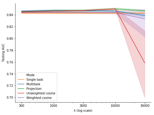
We can compare these results with those for unweighted cosine and weighted cosine on Figure 9. The unweighted cosine curve and the weighted cosine curve are very close to respectively the projection curve and the single task curve for $\lambda \leq 10000$ . However, their testing AUC drops for $\lambda = 30000$ . We can note that the weighted cosine curve falls between the single task curve and the unweighted cosine curve, which comes as no surprise.

Experiments on a Synthetic Dataset

The last series of experiments follows (Chen et al., 2018) and uses a synthetic dataset to control the adequacy of the auxiliary task.

Let:

$f(B, \mathbf{x}) = \tanh(B\mathbf{x})$ where $\tanh(\cdot)$ acts element-wise, $\mathbf{x}$ is a real-valued vector of length $250$ and $B$ is a $100 \times 250$ real-valued matrix.
$B_\mathbb{primary}$ , $B$ and $\epsilon$ be constant $100 \times 250$ real-valued matrices whose elements are drawn IID respectively from $\mathcal{N}(0, 10)$ , $\mathcal{N}(0, 10)$ and $\mathcal{N}(0, 3.5)$ .

The primary task and the auxiliary task consist in approximating respectively $f(B_\mathbb{primary},\cdot)$ and $f(B_\mathbb{auxiliary},\cdot)$ with the quadratic loss function where $B_\mathbb{auxiliary}$ can be equal to:

$B_\mathbb{primary}$ (both tasks are the same)
$B_\mathbb{primary} + \epsilon$ (both tasks are similar)
$B$ (both tasks are unrelated)

For the input data (i.e. $\mathbf{x}$ ), the training set, the validation set and the test set include respectively 1000, 1000 and 10000 vectors whose elements are generated IID from $\mathcal{N}(0, 1)$ . Moreover and as opposed to the previous series of experiments, the training sets are distinct for the primary task and the auxiliary task. If these sets were the same, the auxiliary task wouldn’t add any value when $B_\mathbb{primary} = B_\mathbb{auxiliary}$ .

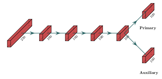
Neural network for the synthetic dataset

Figure 10. Multilayer perceptron with 4 shared layers and an output layer specific to each task, all of them being of size 100

As (Chen et al., 2018), I used the vanilla neural network depicted on Figure 10, which I trained with the Adam algorithm and early stopping.

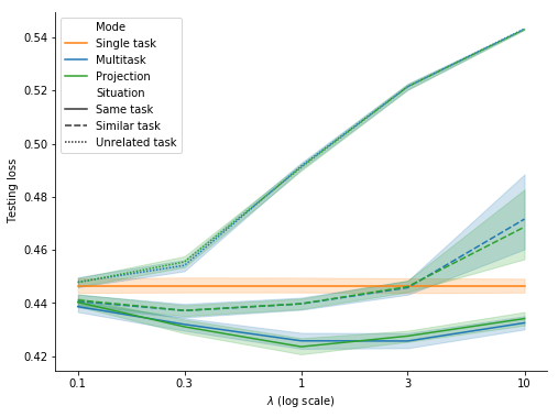
AUC for single task, multitask and projection

Figure 11. Testing loss for single task, multitask and projection for 5 values of $\lambda$ (20 runs for each combination)

Figure 11 shows the results for single task, multitask and projection for various values of $\lambda$ . The outcomes for multitask and projection are almost identical and fully consistent with the 3 situations for the auxiliary task (same task, similar task and unrelated task):

when the auxiliary task is the same as the primary task, it significantly contributes to the performance of the primary task for all 5 values of $\lambda$ .
when the auxiliary task is similar to but different from the primary task, it helps for $\lambda \leq 1$ but becomes neutral or harmful for $\lambda \geq 3$ .
when the auxiliary task is unrelated to the primary task, it’s detrimental to the performance of the primary task for $\lambda \geq 0.3$ .

In contrast to the previous series of experiments, Figure 11 suggests projection has no added value compared to multitask. This difference may result from the fact that the primary task and the auxiliary task don’t share here the same input data. As a consequence, at each optimization step, $\nabla\mathcal{L}_{\text{primary}}$ is less related to $\nabla\mathcal{L}_{\text{auxiliary}}$ and might then be too noisy to help properly adjust it. Therefore I tried substituting $\nabla\mathcal{L}_{\text{primary}}$ with an exponential moving average of $\nabla\mathcal{L}_{\text{primary}}$ for adjusting $\nabla\mathcal{L}_{\text{auxiliary}}$ . With a smoothing constant $0 < \alpha \leq 1$ , $G_{\text{auxiliary}}$ is then given at each optimization step $t$ by:

$G_{\text{auxiliary}}(t) = \nabla\mathcal{L}_{\text{auxiliary}}(t) - \min(0, \nabla\mathcal{L}_{\text{auxiliary}}(t).\frac{M(t)}{||M(t)||})\frac{M(t)}{||M(t)||}$

with $M(0) = \nabla\mathcal{L}_{\text{primary}}(0)$ and $M(t) = \alpha\nabla\mathcal{L}_{\text{primary}}(t) + (1-\alpha)M(t-1)$ for $t > 0$ .

AUC for all modes

Figure 12. Testing loss for single task, multitask and projection for 5 values of $\lambda$ and 3 values of $\alpha$ (20 runs for each combination)

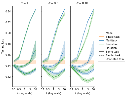
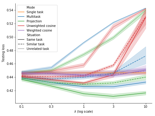
Figure 12 shows the same results as Figure 11 for 3 values of $\alpha$ . With $\alpha = 0.1$ and even more with $\alpha = 0.01$ , projection yields clearly better results compared to multitask for all 3 situations⁵. Figure 13 zooms in on the case $\alpha = 0.01$ , for which unweighted cosine and weighted cosine provide better results than multitask and projection only when the primary task and the auxiliary task are unrelated.

AUC for various scales

Figure 13. Testing loss for single task, multitask, projection, unweighted cosine and weighted cosine for 5 values of $\lambda$ and $\alpha = 0.01$ (20 runs for each combination)

Conclusion

Leveraging auxiliary tasks is an elegant way to improve learning, especially in the case of supervised learning with too few labelled examples or reinforcement learning with sparse rewards. However, auxiliary tasks may sometimes hurt the performance on the primary task.

In this blog post, I proposed a simple and intuitive method to mitigate such risk of negative transfer. I tested it in a few basic scenarios, in which it brought moderate but statistically significant gains over the standard multitask approach. This is a promising start but more diverse and elaborate experimental settings would be necessary to draw general conclusions on this method’s relevance or compare it with its alternatives.

Many thanks to the authors of the inspiring articles listed below and the developers of the great tools used for this post: Tensorflow, the SciPy ecosystem, Seaborn, Google Colab, PlotNeuralNet and Jekyll. Many thanks as well to Sebastian Ruder for his valuable feedback.

References

Caruana, R., Baluja, S., & Mitchell, T. (1996). Using the future to "sort out" the present: Rankprop and multitask learning for medical risk evaluation. Advances in Neural Information Processing Systems, 959–965.
Vincent, P., Larochelle, H., Bengio, Y., & Manzagol, P.-A. (2008). Extracting and composing robust features with denoising autoencoders. Proceedings of the 25th International Conference on Machine Learning, 1096–1103.
Zhang, Z., Luo, P., Loy, C. C., & Tang, X. (2014). Facial landmark detection by deep multi-task learning. In ECCV. 94–108.
Mordan, T., Thome, N., Henaff, G., & Cord, M. (2018). Revisiting Multi-Task Learning with ROCK: a Deep Residual Auxiliary Block for Visual Detection. Advances in Neural Information Processing Systems, 1317–1329.
Trinh, T. H., Dai, A. M., Luong, T., & Le, Q. V. (2018). Learning longer-term dependencies in rnns with auxiliary losses. ArXiv Preprint ArXiv:1803.00144.
Mikolov, T., Sutskever, I., Chen, K., Corrado, G. S., & Dean, J. (2013). Distributed representations of words and phrases and their compositionality. Advances in Neural Information Processing Systems, 3111–3119.
Jaderberg, M., Mnih, V., Czarnecki, W. M., Schaul, T., Leibo, J. Z., Silver, D., & Kavukcuoglu, K. (2016). Reinforcement learning with unsupervised auxiliary tasks. ArXiv Preprint ArXiv:1611.05397.
Burda, Y., Edwards, H., Pathak, D., Storkey, A., Darrell, T., & Efros, A. A. (2018). Large-scale study of curiosity-driven learning. ArXiv Preprint ArXiv:1808.04355.
Du, Y., Czarnecki, W. M., Jayakumar, S. M., Pascanu, R., & Lakshminarayanan, B. (2018). Adapting auxiliary losses using gradient similarity. ArXiv Preprint ArXiv:1812.02224.
Liu, Z., Luo, P., Wang, X., & Tang, X. (2015, December). Deep Learning Face Attributes in the Wild. Proceedings of International Conference on Computer Vision (ICCV).
Chen, Z., Badrinarayanan, V., Lee, C.-Y., & Rabinovich, A. (2018). GradNorm: Gradient Normalization for Adaptive Loss Balancing in Deep Multitask Networks. Proceedings of the 35th International Conference on Machine Learning, ICML 2018, Stockholmsmässan, Stockholm, Sweden, July 10-15, 2018, 793–802. http://proceedings.mlr.press/v80/chen18a.html

The terminology for auxiliary learning is somewhat unclear in the academic litterature. Auxiliary learning may or may not be included in multitask learning depending on the papers. In this post, I restrict multitask learning to the situations where all tasks are taken into account to assess the model’s performance. Consequently multitask learning is here disjoint from auxiliary learning. ↩
Sebastian Ruder presents this approach as well as other approaches in his very good overview of multitask learning. ↩
$\lambda$ varies in certain methods not presented here. Transfer learning can be seen as a specific case for which $\lambda = \infty$ in a first stage and $\lambda = 0$ in a second stage. ↩
As an extreme example, an auxiliary task identical to the primary task and yielding the same gradients would be unhelpful provided that the learning rate is appropriately tuned. ↩
It may be surprising that multitask isn’t the best training mode when the primary task and the auxiliary task are the same. In fact, the situation isn’t fully symmetrical because the primary task helps train the corresponding task-specific last layer which isn’t affected by the auxiliary task. ↩

Written on February 17th, 2019 by Vivien

Feel free to share!